hawkee

Featured

LLMs are Slaves to the Law of Large Numbers

New preprint: https://arxiv.org/abs/2405.13798

We propose a new asymptotic equipartition property for the perplexity of a large piece of text generated by a language model and present theoretical arguments for this property. Perplexity, defined as a inverse likelihood function, is widely used as a performance metric for training language models. Our main result states that the logarithmic perplexity of any large text produced by a language model must asymptotically converge to the average entropy of its token distributions. This means that language models are constrained to only produce outputs from a “typical set”, which we show, is a vanishingly small subset of all possible grammatically correct outputs. We present preliminary experimental results from an open-source language model to support our theoretical claims. This work has possible practical applications for understanding and improving “AI detection” tools and theoretical implications for the uniqueness, predictability and creative potential of generative models.

Claude Shannon on AI slop

From his famous Bandwagon editorial in 1956:

Secondly, we must keep our own house in first class order. The subject of information theory has certainly been sold, if not oversold. We should now turn our attention to the business of research and development at the highest scientific plane we can maintain. Research rather than exposition is the keynote, and our critical thresholds should be raised. Authors should submit only their best efforts, and these only after careful criticism by themselves and their colleagues. A few first rate research papers are preferable to a large number that are poorly conceived or half-finished. The latter are no credit to their writers and a waste of time to their readers. Only by maintaining a thoroughly scientific attitude can we achieve real progress in communication theory and consolidate our present position.

Can you measure the built-in potential of a pn junction?

When we talked about the built-in barrier potential of a pn junction, perhaps you thought about measuring it on a disconnected diode in the lab. (Even if you didn’t think of it, you should go ahead and try it). You will find that it doesn’t work. It is worth thinking about why i.e. why can’t you measure the built-in potential of a pn junction with a simple voltmeter (or why do we need a special diode mode in a multimeter)?

At one level, it is easy to see why this can’t work: a bare diode cannot drive a current (that would be needed to measure a voltage in a voltmeter), because that would require the diode to supply power which would effectively make it a perpetual motion machine. (If you are unfamiliar with perpetual motion, treat yourself to a tour of the work of the Dutch artist M.C. Escher.)

But I don’t find this entirely satisfactory. In particular, we should still be able to show how, for instance, to explain the voltmeter measurement in terms of the Kirchoff voltage law. For some interesting discussions of this question see here and here. I find the below quote from this forum very appealing:

In a simple idealized view, the Fermi level is the top energy level in the solid occupied by electrons. In silicon with no doping it sits at mid-gap: the valance band is full, the conduction band empty. In a thought experiment, if you had two separate chunks of intrinsic silicon each would be perfectly happy in isolation. If you could mash them together to make a “junction”, everything would still be perfectly happy – the Fermi levels line up, and no electron has any real desire to do something else.

Adding dopants shifts the Fermi level. In n-doped material there are newly available occupied levels near the conduction band edge, and in p-doped materials there are newly available un-occupied levels near the valance band. By doping the material you have fixed the Fermi level at a new point. In isolation, the n-doped chunk is happy, and the p-doped chunk is happy. Here, though, when you mash them together to make the junction, they realize that together they aren’t happy. The occupied levels on the n-doped side are above empty levels in the p-doped side: this is a non-equilibrium condition since electron (hole) flow will reduce the energy of the system. But wait! Indeed, the electrons (holes) start sloshing around, but in doing so they leave behind the dopants. These now-abandoned dopants have a net charge, and an internal field begins to build up. It will build up until it is large enough to prevent further electron (hole) flow across the junction. However, an equivalent view is that this built in voltage is just what is needed to bring the different Fermi levels into alignment (as in @boyfarrell’s picture above). (I find the water analogy a bit misleading, since it is the separation of fixed dopants and moving charges that leads to the build-in voltage.)

So, ultimately, yes: the built-in voltage is precisely what makes the p-n junction in equilibrium with no net potential across the terminals.

Circuits Numeracy

Let’s talk about numbers in circuits. Our goal is to develop numeracy:

More precisely, we want to develop a sense for scale i.e. a sense for what kind of numbers are physically reasonable.

We all have an intuitive sense of scale for the physical world. More precisely, we can very easily tell when physical quantities are absurdly large or small. As an example, if we are asked to estimate the weight of a bag of apples, we know immediately that 50 mg or 5000 kg are both absurd numbers. However, because the electrical world is more abstract and not directly accessible to our senses, such intuition is not naturally acquired, but instead must be deliberately cultivated.

In the PEI class, we are concerned with a class of “low frequency” electronic circuits. What frequencies are considered “low”? Specifically this means circuits where the timescale of voltage and current fluctuations is slow enough that transmission line effects can be neglected. This means that we can neglect the fact that electrical disturbances travel at the speed of light which is approximately 1 ft/ns. A sine wave at a frequency of 100 MHz has an oscillation time of 10 ns. At frequencies higher than this (with shorter oscillation times), the finite speed of light cannot be ignored; wires no longer behave like short-circuits nor air gaps as open circuits. This is the regime of RF and microwave circuit design. In our class, we work with frequencies of 10 MHz or less where we can comfortably ignore such “high frequency” effects.

Time. So this is a good place to start: for timescales, in our class we are concerned with timescales significantly longer than 10 ns, and usually shorter than 100 ms or so.

Voltage and current. Voltages are usually within a couple of orders of magnitude of 1 V i.e. 10 mV is a very small voltage and 100 V is fairly large. A Volt is an excellent unit for voltage. Sadly the Amp is a poor unit for current: 1 A is a very large current! 1 mA is a much more comfortable unit and we usually work with currents within a couple of orders of magnitude of this.

Resistance. Once we have the above, it is a matter of simple dimensional analysis (which is a valuable tool for numeracy – learn it!) to figure out reasonable range of values for other circuit quantities. We will illustrate with resistance. A small resistance would produce a small voltage drop even with a fairly large current e.g. 50 mV with 50 mA of current. Thus 1 $\Omega$ is a very small resistance – the Ohm is a poor unit for resistance!

What can you infer about other quantities such as charge, energy, power, capacitance and inductance?

Are holes real?

Charge transport by holes is an important concept in semiconductor physics. In particular, it is important to understand charge transport by holes as different and separate from charge transport by electrons.

What makes this a tricky concept is that holes are generally described as the absence of an electron or slightly less informally as unoccupied electron energy states. In this view, holes are simply a convenient short-hand: when we talk of holes moving, it is simply an indirect description of an electron moving in the opposite direction.

So are holes real?

This is a much more subtle question than it may initially appear.

First of all, while it may seem lawyerly, at some level you do need to encounter the philosophical question of what it means for something to be “real”. See e.g. here, here and here.

As engineers, we would prefer to avoid such intractable questions. One possible approach is to avoid the question entirely: holes are a useful construct and that’s all that matters. An alternative, pragmatic approach is to treat holes as real to the extent we are able to observe and manipulate them in the same way that we observe and manipulate, say, electrons, which we know to be real (how?).

And this is where things get interesting: it turns out that you can observe holes in a very direct and satisfying manner using an elegant but simple experiment:

Some additional discussions of this question are here and here.

Diffusion Models – 1: The Surprisingly Tricky Kolmogorov Equations

This is the first of a series of notes to understand the mathematics of diffusion models from the perspective of an electrical engineer with a background in the mathematical theory of signals and systems based on frequency domain analysis and the Fourier Transform.

Consider a stochastic process $X(t)$ and let $p(x_2, t_2|x_1, t_1) \doteq \Pr \left( X(t_2)=x_2 | X(t_1)=x_1 \right)$ , be the conditional probability that the process takes the value $x_2$ at time $t_2$ given $X(t_1)=x_1$ .

From The Law of Total Probability, we have $p(x_2, t_2) \equiv \int_{x_1} p(x_2, t_2|x_1, t_1) p(x_1, t_1) d x_1$ . This holds for all $x_1, t_1, x_2, t_2$ , but we will now specialize to a causal sequence of time instants $t_0 < t_1 < t_2$ and so on. Again using The Law of Total Probability, we can write: $p(x_2, t_2 | x_0, t_0) \equiv \int_{x_1} p(x_2, t_2|x_1, t_1, x_0, t_0) p(x_1, t_1|x_0, t_0) d x_1$ .

If we add the assumption that $X(t)$ is Markov, we get a (slightly) simplified equation: $p(x_2, t_2 | x_0, t_0) \equiv \int_{x_1} p(x_2, t_2|x_1, t_1) p(x_1, t_1|x_0, t_0) d x_1$ which is sometimes called the Master Equation (ME) – a rather grandiose name for a fairly humble observation.

Differential Form of the Master Equation

Now we will limit ourselves to continuous-time, continuous-valued process $X(t)$ that are nice and smooth. Specifically, we will assume that $X(t)$ is continuous. Of course, for random processes, there are many different definitions of continuity, but we will adopt an informal definition: over an infinitesimally small time intervals $\Delta t$ , the change $\Delta X(t)$ must also be infinitesimally small. Specifically, we will assume that $p(x_2, t+ \Delta t|x_1, t)$ is zero for all values of $x_2$ except a small neighborhood $\left|x_2-x_1 \right| \leq \Delta x$ . The same is true of course of the product $p(x_2, t_2|x_1, t_1) p(x_1, t_1)$ . A standard method in the theory of stochastic processes is represent this product by a Taylor Series to obtain the so-called Kramers-Moyal expansion to express the Master Equation in a differential form. A truncation of this Taylor Series yields the famous Fokker-Planck equation.

However, a detailed derivation of this Taylor Series turns out to be surprisingly tricky if we want to maintain full generality and avoid additional simplifying assumptions.

A Wrong Turn

Consider $p(x,t+\Delta t) \equiv \int_{x_1 = -\infty}^\infty p(x, t + \Delta t|x_1, t) p(x_1, t) d x_1$ . Let $\epsilon \doteq x-x_1$ be the (random) increment in $X(t)$ in the time interval $\Delta t$ . It is tempting to try $p(x,t+\Delta t) \equiv -\int_{\epsilon= -\infty}^\infty p(x, t + \Delta t|x - \epsilon, t) p(x-\epsilon, t) d \epsilon$ and write a Taylor Series for the integrand. This, however, is a road to nowhere: Taylor Series are useful over a limited range of values for $\epsilon$ , but this formulation requires integrating over all $\epsilon \in \mathbb{R}$ .

One way to salvage this attempt is to assume the process $X(t)$ has independent increments so the transition probabilities are state-independent i.e. $p(x, t + \Delta t|x - \epsilon, t) \equiv p(\epsilon, t + \Delta t|0, t) \equiv p_t(\epsilon)$ . According to our previous smoothness assumption, the fixed distribution $p_t(\epsilon)$ has finite support in $\epsilon \in [-\Delta x,\Delta x]$ , and so we can write $p(x,t+\Delta t) \equiv -\int_{\epsilon= -\Delta x}^{\Delta x} p_t(\epsilon) p(x-\epsilon, t) d \epsilon$ . Over this small and finite range, we can perform a Taylor expansion of $p(x-\epsilon, t)$ .

However, the independent-increments assumption represents a rather significant loss of generality, so we will see if we can avoid this. Our salvage attempt suggests a way forward: keep the $p(x, t + \Delta t|x_1, t)$ term and only do a Taylor expansion of the other term $p(x_1, t) \equiv p(x-\epsilon,t)$ . Thus, we have for the first two Taylor Series terms: $p(x,t+\Delta t) \equiv -\int_{\epsilon= -\Delta x}^{\Delta x} p(x, t + \Delta t|x - \epsilon, t) \left( p(x, t) -\epsilon p'(x,t) + \dots \right) d \epsilon$ .

Unfortunately, this expression cannot be simplified because the term $p(x, t + \Delta t|x - \epsilon, t)$ is not a distribution over the variable of integration $\epsilon$ . With a clever modification, we can make this derivation much more tractable.

A More Careful Attempt

Define $f_\epsilon(x)=p(x+\epsilon, t + \Delta t|x, t) p(x, t)$ . The subscript in $f_\epsilon(x)$ is to remind ourselves that it is defined for a specific value of $\epsilon$ . Then we have $p(x,t+\Delta t) \equiv -\int_{\epsilon=-\infty}^\infty f_\epsilon(x-\epsilon) d\epsilon$ .

Now consider the expansion $f_\epsilon(x-\epsilon)=f_\epsilon(x)-\epsilon f'_\epsilon(x)+\frac{\epsilon^2}{2}f''_\epsilon(x)+\dots$ , We have to determine if this avoids the pitfalls that we ran into in our earlier attempts. First, note that $\int_{\epsilon} f_\epsilon(x) d\epsilon \equiv p(x,t)$ . Define $a_{\Delta t}(x,t) \doteq \int_{\epsilon} \epsilon f'_\epsilon(x) d\epsilon \equiv \int_\epsilon \epsilon p(x+\epsilon, t + \Delta t|x, t) d\epsilon$ and $b_{\Delta t}(x,t) \doteq \int_{\epsilon} \frac{\epsilon^2}{2} f''_\epsilon(x) d\epsilon \equiv \int_\epsilon \frac{\epsilon^2}{2} p(x+\epsilon, t + \Delta t|x, t) d\epsilon$ .

We have: $p(x,t+\Delta t) \equiv p(x,t)+\frac{\partial}{\partial x} \Big( p(x, t) a_{\Delta t}(x,t) \Big) + \frac{\partial^2}{\partial x^2} \Big( p(x, t) b_{\Delta t}(x,t) \Big) + \dots$ . Note that both $a_{\Delta t}(x,t),~b_{\Delta t}(x,t)$ vanish as $\Delta t \rightarrow 0$ and the limits $a(x,t) \doteq \frac{1}{\Delta t}a_{\Delta t}(x,t),~b(x,t) \doteq \frac{1}{\Delta t}b_{\Delta t}(x,t)$ when they are non-zero have natural physical interpretations as the drift rate and diffusion rate of the process $X(t)$ .

Thus we finally have the famous Fokker-Planck equation also known as the Kolmogorov forward equation: $\frac{\partial p(x,t)}{\partial x} \equiv \frac{\partial}{\partial x} \Big( p(x, t) a(x,t) \Big) + \frac{\partial^2}{\partial x^2} \Big( p(x, t) b(x,t) \Big)$ by keeping only the first two terms in the Taylor expansion.

The Gaussian distribution — 4: Conditioning like a Pro

In Part 3, we introduced the important and powerful idea of applying geometric ideas about vectors in 2D and 3D space to complex mathematical objects such as random variables and waveforms. We will now show how to use these geometric ideas to understand and visualize an important and frequently-used method in Bayesian inference: finding the conditional distribution of one set of Gaussian rvs given another.

We will work with the example of a simple Markov chain to illustrate these ideas. Consider iid standard Gaussian rvs $X_1,~X_2,~X_3 \sim N(0,1)$ , and the Markov chain $Y_1 \rightarrow Y_2 \rightarrow Y_3$ of Gaussian rvs $\underline{Y} = [Y_1,~Y_2,~Y_3]^T$ where $Y_1 \doteq X_1;~Y_2 \doteq X_1 + X_2;~Y_3 \doteq X_1+X_2+X_3$ .

Clearly, $\underline{Y}$ has zero mean and the covariance: $C_{\underline{Y}} \equiv \begin{pmatrix} 1 & 1 & 1 \\ 1 & 2 & 2 \\ 1 & 2 & 3 \end{pmatrix}$ . The lengths of the three vectors are $|Y_1| \equiv \sigma_1 = 1,~|Y_2| \equiv \sigma_2 = \sqrt{2},~|Y_3| \equiv \sigma_3 = \sqrt{3}$ . The correlation coefficient between $Y_1,~Y_2$ is $\rho_{12} = \frac{C_{12}}{\sigma_1 \sigma_2} \equiv \frac{1}{\sqrt{2}}$ and the angle between them is $\theta_{12} \equiv \cos^{-1} \left( \rho_{12} \right) = 45^\circ$ . Likewise for $Y_2,~Y_3$ we have $\rho_{23} = \frac{C_{23}}{\sigma_2 \sigma_3} \equiv \sqrt{\frac{2}{3}}$ and the angle between them is $\theta_{23} \equiv \cos^{-1} \left( \rho_{23} \right) = 35.2^\circ$ and so on.

Conditioning: an easy example. As a warm-up exercise, let us find the conditional distribution of $Y_2,~Y_3$ given $Y_1=a$ . This is straightforward because knowing $Y_1=a$ tells us that $X_1=a$ , but since $X_2,~X_3$ are independent of $X_1$ , their distributions do not change. Thus we have $Y_2|_{Y_1=a}=a+X_2,~Y_3|_{Y_1=a}=a+X_2+X_3$ . The conditional means of $[Y_2,~Y_3]^T$ is $[a,~a]^T$ and their conditional covariance is $\begin{pmatrix} 1 & 1 \\ 1 & 2 \end{pmatrix}$ .

Brute-Force Method. Now let’s find the conditional distribution of $Y_1,~Y_2$ given $Y_3=c$ . This is not as straightforward as the previous case because $Y_3$ is correlated with all three of $X_1, X_2, X_3$ and all of their distributions will change when we condition on $Y_3=c$ .

We can, of course, always find the conditional distribution algebraically using the known joint and marginal distributions as $f_{Y_1,Y_2|Y_3}\left( y_1, y_2 | Y_3=c \right) \equiv \frac{f_{Y_1, Y_2, Y_3}(y_1,y_2,c)}{f_{Y_3}(c)}$ . But we want to avoid this brute-force approach and would like to find a more elegant, intuitive method. We now show how to do this using geometric manipulations with vectors.

Conditioning Elegantly. Consider the figures below that shows the geometric relationship between $Y_3,~Y_1$ and $Y_3,~Y_2$ . (Note that we cannot show all three vectors representing $Y_1, Y_2, Y_3$ on the same planar vector diagram and preserve geometric relationships such as angles; this is because the three rvs are linearly independent which means the corresponding vectors are not coplanar.)

The key idea is to project the vector $Y_1$ in the direction of $Y_3$ , so that we can express $Y_1 = Y'_3+W_1$ as the sum of two component vectors, one $Y'_3$ that is perfectly aligned with $Y_3$ and the other perfectly orthogonal to $Y_3$ . By definition, $Y'_3 = \gamma Y_3$ for some constant $\gamma$ . We need to find this constant in terms of the statistics of $Y_1,~Y_3$ .

Projection using Basic Trigonometry. We now show how to do this using very elementary geometric arguments. Let $\hat{u}_3 \doteq \frac{1}{\sigma_3} Y_3$ denote the unit vector in the direction of $Y_3$ . By definition, $Y'_3 \equiv |Y'_3| \hat{u}_3$ . From the trigonometry of the right-angled triangle formed by the vectors $Y'_3, W_1, Y_1$ , we have $|Y'_3| = |Y_1| \cos \theta_{13} \equiv \sigma_1 \rho_{13}$ and $|W_1| = |Y_1| \sin \theta_{13} \equiv \sigma_1 \sqrt{1-\rho_{13}^2}$ which gives $\gamma \equiv \frac{\sigma_1}{\sigma_3} \rho_{13} = \frac{1}{3}$ and $\sigma_{W_1}^2 \equiv \sigma_1^2 \left( 1-\rho_{13}^2 \right) = \frac{2}{3}$ .

Thus we have $Y_1 = \frac{1}{3} Y_3 + W_1$ , where $W_1$ is independent of $Y_3$ . Therefore $Y_1|_{Y_3=c} = \frac{1}{3} c + W_1 \sim N \left( \frac{1}{3}c, \frac{2}{3} \right)$ . Similarly, we can show that $Y_2|_{Y_3=c} = \frac{2}{3} c + W_2 \sim N \left( \frac{2}{3}c, \frac{1}{3} \right)$ .

Conditional Covariance. We have almost completed the task we set ourselves: to find the conditional distribution of $Y_1,~Y_2$ given $Y_3=c$ . In particular, we have now calculated the means and variances of $Y_1,~Y_2$ and therefore the conditional marginal distributions of $Y_1,~Y_2$ given $Y_3=c$ . However, to find the conditional joint distribution of $Y_1,~Y_2$ , we also need to find their conditional covariance. This is easily done as follows: $C_{1,2|3} = E \left( W_1 W_2 \right) \equiv E \left( \left( Y_1 - \frac{Y_3}{3} \right) \left( Y_2 - \frac{2Y_3}{3} \right) \right)$ . Note that since both $W_1,~W_2$ are independent of $Y_3$ , this expectation is unaffected by conditioning on $Y_3=c$ and is easily evaluated as: $C_{1,2|3} \equiv C_{\underline{Y}}(1,2) - \frac{2}{3} C_{\underline{Y}}(1,3) - \frac{1}{3} C_{\underline{Y}}(2,3) + \frac{2}{9} C_{\underline{Y}}(3,3) \equiv \frac{1}{3}$ .

These ideas can be generalized in a fairly straightforward way to conditioning on multiple random variables and these generalizations form the core of some very important and powerful techniques in statistical inference. A famous example of such a technique is the Kalman Filter. We will conclude this topic with a summary and a few further comments about applications in Part 5.

The Gaussian distribution — 3: Vector Apples and Oranges

In Part 1 of this series, we presented a simple, intuitive introduction to the Gaussian distribution by way of the Central Limit Theorem. In Part 2, we introduced multi-variate Gaussian distributions, and also looked at certain weird ways of constructing Gaussian random variables that are not jointly Gaussian. If we disregard these “unnatural” mathematical constructions and limit ourselves to natural Gaussians i.e. jointly-Gaussian random variables, we can take advantage of certain simple geometric methods to do important and powerful mathematical operations such as constructing conditional distributions.

Abstract Theory of Vector Spaces. We all have an innate geometric intuition with 2D and 3D space. Electrical Engineers encounter 2D and 3D vectors whenever we work with EM fields or Maxwell’s Equations. Mathematicians however, have developed a general and abstract theory of vector spaces in which certain geometric ideas from working with vectors in 2D and 3D space can be generalized and applied to fairly complex mathematical objects.

Two such mathematical objects are of special interest to us: (a) random variables, and (b) waveforms; in both cases, an inner-product operation that satisfies the Cauchy-Schwartz Inequality can be defined. This operation serves the same role as the dot-product for 2D and 3D vectors; in particular it allows us to define the angle between two of these objects, which in turn allows us to define projections and orthogonality.

Random Vectors v. Random Variables as Vectors. As noted above, many different types of mathematical objects can be considered as elements of some abstract vector space. It is important, of course, not to mix together vectors representing different kinds of mathematical objects. E.g. we cannot add a vector representing a waveform to a vector representing a random variable. They are like apples and oranges and they belong to different spaces.

When working with Gaussian rvs, we may encounter different types of vectors. For example, we often find it convenient to organize a collection of related random variables into a random vector. Thus we may define a random vector $\underline{X} \doteq [X_1,~X_2,~\dots, X_N]^T$ as a column vector with joint Gaussian rvs $X_i$ as elements. Clearly, $\underline{X} \in \mathbb{R}^N$ . We may use the distribution $f_{\underline{X}}(\underline{x})$ as a short-hand for the joint distribution of the $X_i$ ‘s and so on.

At the same time, if the $X_i$ ‘s are zero mean, they can each be considered elements in an abstract vector space $\mathcal{X}$ of random variables. Of course, being random variables, each of the $X_i$ ‘s take real-number values.

Angle Between Two Random Variables. In its vector representation, the length of a random variable is its standard deviation. The correlation coefficient between two random variables serves as the inner product; it is interpreted as a measure of the alignment between two vectors. A zero correlation coefficient means two vectors are orthogonal; the corresponding rvs are uncorrelated, which for Gaussian rvs means they are independent. The lengths of orthogonal vectors obey the Pythagoras Theorem and the usual trigonometric equations. In the diagram below, $X_1 \sim N(0,\sigma_1^2),~X_2\sim N(0,\sigma_2^2)$ are jointly Gaussian rvs represented by vectors of lengths $\sigma_1,~\sigma_2$ respectively. The angle between them is related to the correlation coefficient as $\rho\equiv \cos \theta$ .

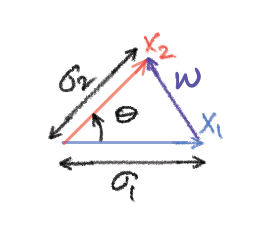
From the relationship between the vectors in the diagram, we can see that the random variable $W \equiv X_2-X_1$ . Its variance can be calculated algebraically as $\sigma_w^2 \doteq E \left( \left( X_2-X_1 \right)^2 \right) \equiv \sigma_1^2+\sigma_2^2-2 \rho \sigma_1 \sigma_2$ . It is easily checked that this matches exactly the well-known elementary geometric relationship between the sides of a triangle: $|W|^2 = |X_1|^2+|X_2|^2-2|X_1||X_2|\cos \theta$ .

This vector representation is very useful for an intuitive understanding of dependencies between Gaussian random variables. In particular, the geometric concept of orthogonal projection allows us to visualize an important idea in Bayesian inference: the conditional distribution of one set of Gaussian random variables given another. This is the topic for Part 4.

The Gaussian distribution — 2: Frankenstein Monsters

In Part 1, we introduced the Gaussian distribution as naturally arising from the mixing of a large number of independent random variables. Random mixing has an averaging effect that can be described by a sequence of approximations. As a first order approximation, random mixing reduces the size of fluctuations; asymptotically, the sample average of iid random variables converges to the mean. If we zoom into the small deviations of the mixture around its mean for a second-order approximation, we discover that the deviations converge to a Gaussian. distribution regardless of the distribution of the underlying random variables. This is the famous Central Limit Theorem (CLT).

Once you go Gaussian… In addition to its ubiquity in nature, the popularity of the Gaussian distribution can also be attributed to its many, very nice mathematical properties which makes us want to use these distributions. First and most important, mixtures of independent Gaussian random variables are also Gaussian. From our previous reasoning that led up to the CLT, this should be unsurprising.

Consider a sequence of iid standard Gaussian random variables collected into a column vector $\underline{Z} \doteq [Z_1, Z_2 \dots Z_M]^T$ , and a sequence of derived random variables $\underline{X} = A \underline{Z}$ , where A is a $N \times M$ matrix. Thus $\underline{X} \doteq [X_1, X_2 \dots X_N]^T$ is a sequence of random variables that are linear combinations of the $Z_i$ ‘s.

Natural Gaussians. By the previous reasoning, the $X_i$ ‘s are all Gaussian. Furthermore, all linear mixtures of the $X_i$ ‘s are also Gaussian. Note however, that the $X_i$ ‘s are not in general independent of each other; they depend on each other through a shared dependence on one or more of the underlying independent variables $Z_i$ .

We call such random variables $X_i$ multi-variate Gaussian or jointly Gaussian, but they could also be reasonably called natural Gaussians. Indeed, there is a multi-variable version of the Central Limit Theorem that shows how a set of multi-causal random variables that are each an aggregate of a large number of independent random variables converge to a multi-variable generalization of the single-variable Gaussian distribution regardless of the underlying distributions.

But calling these natural Gaussians begs the question: is there another kind?

Gaussians with .. Unnatural Dependencies. Sometimes the nice mathematical properties of the Gaussian distribution can lead to .. annoying mathematical corner cases. We can take two iid standard Gaussian rvs $Z_1, Z_2$ and create nice, little baby Gaussians like e.g. $X_1 = Z_1 - Z_2,~X_2 = 2 Z_1 + Z_2$ . These are the nice, natural kind of Gaussians we discussed above.

But we can also create weird Frankenstein monster Gaussians like $V_1 = Z_1 \mathrm{sgn}(Z_2)$ where $V_1$ is equal to $\pm Z_1$ depending on the sign of $Z_2$ . Randomly flipping the sign of a zero mean Gaussian still yields a Gaussian rv because of the even symmetry of the Gaussian density function. The new rv $V_1$ is uncorrelated with $Z_1$ , but certainly not independent of it. The mixture $V_1+Z_1$ is very far from a Gaussian: it is zero with 50% probability!

While there are numerous ways to cook up this kind of weird Gaussian random variables, they almost never exist in the wild.

If we limit ourselves to the nice kind of multi-variate Gaussians, we can apply some very nice and intuitive geometric ideas to them. That’s a topic for Part 3.

Informal Introduction to the Gaussian Distribution – 1: Central Limits

Consider a random variable X obtained from a random experiment E with the mean, variance $\mu,~\sigma^2$ and density function $f_X(x)$ .

First- and Second-order approximations. The mean and variance provide a simple, partial statistical description of the random variable X that is easy to understand intuitively: the mean is the center of mass of the distribution $f_X(x)$ , while the standard deviation $\sigma$ is a measure of the spread of the distribution away from the mean. The complete statistical description of X is of course provided by the density function $f_X(x)$ .

Specifying a distribution by its moments. An alternative statistical description of a random variable is in terms of its moments: $\mu_n^n \doteq E \left[ X^n \right],~n=1,2, \dots \infty$ . To understand the moments of a distribution intuitively, consider the characteristic function $\Phi_X(\omega) \doteq E \left[ e^{j \omega X} \right]$ . Mathematically, the characteristic function is the Fourier transform of the density function $f_X(x)$ . For low “frequencies” $\omega$ , we can approximate the characteristic function by a Taylor Series: $\Phi_X(\omega) \equiv 1 + j\omega \mu - \frac{1}{2} \omega^2 \left( \mu^2 + \sigma^2 \right) - \frac{1}{3!} j \omega^3 \mu_3^3 + \dots$ .

Roughly speaking, the lower-order moments provide a coarse, “low frequency” approximation to the distribution, and higher-order moments supply finer-grained “high-frequency” details.

The Law of Large Numbers. Consider N independent repetitions of the experiment E resulting in the iid sequence of random variables $X_1,~X_2,~\dots,~X_N$ . The sample mean random variable $S \doteq \frac{1}{N} \sum_{I=1}^N X_i$ has the mean $\mu$ and variance $\frac{\sigma^2}{N^2}$ .

Clearly, since the variance of S vanishes as $N \rightarrow \infty$ , the random variable S converges to its mean. This is also easily confirmed from $\Phi_S(\omega) \equiv \left ( \Phi_X \left( \frac{\omega}{N} \right) \right)^N \equiv \left ( 1 + j \frac{\omega}{N} \mu - \frac{1}{2} \frac{\omega^2}{N^2} \left( \mu^2 + \sigma^2 \right) + \dots \right)^N \rightarrow e^{j \omega \mu}$ . This is one version of the famous Law of Large Numbers (LLN).

Deviations from the Mean. The LLN represents a first-order approximation to the distribution of the sample mean S. To refine this approximation and look at how S is distributed around its mean, consider the “centered random variable” $\tilde{Y} \doteq S - \mu \equiv \frac{1}{N} \sum_{I=1}^N \left( X_i - \mu \right)$ . This random variable has the characteristic function $\Phi_{\tilde{Y}}(\omega) \equiv \left ( 1 - \frac{1}{2} \frac{\omega^2}{N^2} \sigma^2 + \dots \right)^N \rightarrow 1$ . This is simply the LLN all over again i.e. $\tilde{Y} \rightarrow 0$ . It turns out that deviations from the mean, being second-order effects, are small and vanish asymptotically!

Central Limits. To prevent the deviations from the sample mean from becoming vanishingly small, we must magnify or zoom into them explicitly. Thus, we are led to define $Y \doteq \sqrt{N} \left( S - \mu \right) \equiv \frac{1}{\sqrt{N}} \sum_{I=1}^N \left( X_i - \mu \right)$ . This random variable has zero mean and variance $\sigma$ which is finite and its characteristic function is: $\Phi_Y(\omega) \equiv \left ( 1 - \frac{1}{2} \frac{\omega^2}{N} \sigma^2 + \dots \right)^N \rightarrow e^{- \frac{1}{2} \omega^2 \sigma^2}$ .

This is a version of the famous Central Limit Theorem (CLT) that says that the small deviations around the sample mean of a large number of independent random variables $X_i$ follow a Gaussian distribution regardless of the actual distribution of the $X_i$ ‘s!

Random Mixing Smooths over Fine Details. In fact our simple derivation above does not require that the $X_i$ ‘s be identically distributed; only that they have the same mean and variance and that they are independent.

The CLT may help explain why the Bell Curve of the Gaussian distribution is so ubiquitous in nature: for complex, multi-causal natural phenomena, when we look at the aggregate of many small independent variables, the fine details of the underlying variables tend to get obscured.

There are many Internet resources that provide nice illustrations of the CLT. Here’s one from this website:

However, it is important to recognize that the CLT is an asymptotic result and usually applies in practice as an approximation. Following the logic of the derivation above, we should expect the CLT to only account for the coarse features of the distribution; in particular, the Gaussian approximation should not be relied on to predict the probability of rare “tail events”.

One place where the Gaussian approximation works really well is for the distribution of noise voltages in circuits. This is understandable when the noise is thermal in origin. Of course noise voltages are random waveforms, and their statistical description is more complex than that of a single random variable. In particular, we need to discuss the joint distribution of multiple Gaussian random variables or equivalently, Gaussian random vectors. This is a topic for Part 2.