Thinking about ideal op-amps

In your previous Circuits class, you were introduced to ideal op-amp circuits. In our class this semester, we will be building on this and become familiar with a small number of simple, but very useful op-amp circuits (e.g. inverting and non-inverting feedback amplifiers, integrators, adders and a few variants of these). Meanwhile we have been doing some HW problems to refresh your knowledge of ideal op-amps. Here’s a quick summary of what you need to know.

First thing to know about op-amps is that though their ideal circuit behavior can be described in very simple terms, they are quite complex internally. How complex? Here’s a look at the internals of a classic model (which we may return to later in class if we have time). This complexity is unlike other circuit elements such as sources, resistors, capacitors and transformers that you learned about in your previous class. At this point, we do not know how to analyze arbitrary op-amp circuits even under ideal conditions, much less design them; a naively designed op-amp circuit can easily show instability.

All we know how to do is to solve approximately for voltages and currents in a class of negative feedback op-amp circuits that we trust to be stable and within their operating limits with DC (or low frequency) inputs. Even this limited knowledge can be extremely valuable, but it is wise to be appropriately humble about this.

A simple model for an op-amp is shown in this figure (from here):

The input currents are both very small (ideally zero), and the gain A very large (ideally ). Thus, a very small voltage difference at the op-amp inputs can produce a large output voltage .

In the kind of circuits we are interested in, the op-amp “looks” at the output voltage through a feedback connection and adjusts the output voltage and current to be whatever they need to be, to force the currents and voltage difference at the input terminals to be zero i.e. . In other words, the op-amp adjusts its output voltage and current in such a way that the input terminals look simultaneously like an open circuit and a short circuit! It is very elegant and almost seems magical when you set it up correctly.

And this is all you need to know to solve the kind of op-amp circuits we will encounter this semester! Sort of…

Unfortunately, it is too easy to get carried away by the simplicity of the ideal op-amp model, which is how you end up with this sloppy example (from your official textbook from Circuits class!):

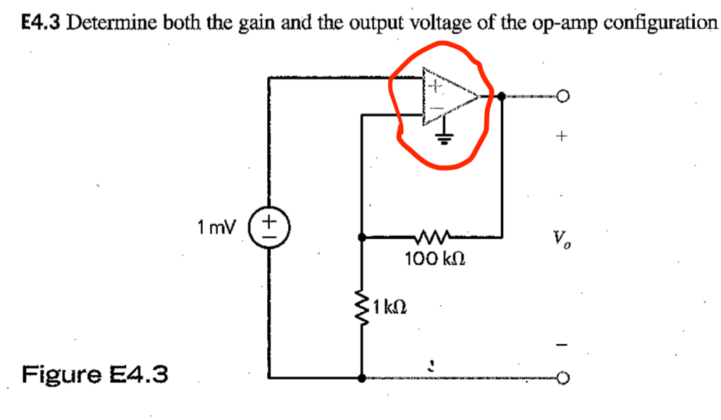
It is easy enough to analyze this circuit using the ideal op-amp model: the op-amp “looks” at the output voltage at the inverting input through the feedback network which is basically a simple voltage divider: . The op-amp then forces the output voltage to be whatever it needs to be to make .

But can you see what’s wrong (or missing) in the schematic above that may cause this circuit to not work as you may expect? (Hint. Can you use a KCL around the red surface surrounding the op-amp and argue that the output current must always be zero? What, if anything, is wrong with that argument?)