The Gaussian distribution — 3: Vector Apples and Oranges

In Part 1 of this series, we presented a simple, intuitive introduction to the Gaussian distribution by way of the Central Limit Theorem. In Part 2, we introduced multi-variate Gaussian distributions, and also looked at certain weird ways of constructing Gaussian random variables that are not jointly Gaussian. If we disregard these “unnatural” mathematical constructions and limit ourselves to natural Gaussians i.e. jointly-Gaussian random variables, we can take advantage of certain simple geometric methods to do important and powerful mathematical operations such as constructing conditional distributions.

Abstract Theory of Vector Spaces. We all have an innate geometric intuition with 2D and 3D space. Electrical Engineers encounter 2D and 3D vectors whenever we work with EM fields or Maxwell’s Equations. Mathematicians however, have developed a general and abstract theory of vector spaces in which certain geometric ideas from working with vectors in 2D and 3D space can be generalized and applied to fairly complex mathematical objects.

Two such mathematical objects are of special interest to us: (a) random variables, and (b) waveforms; in both cases, an inner-product operation that satisfies the Cauchy-Schwartz Inequality can be defined. This operation serves the same role as the dot-product for 2D and 3D vectors; in particular it allows us to define the angle between two of these objects, which in turn allows us to define projections and orthogonality.

Random Vectors v. Random Variables as Vectors. As noted above, many different types of mathematical objects can be considered as elements of some abstract vector space. It is important, of course, not to mix together vectors representing different kinds of mathematical objects. E.g. we cannot add a vector representing a waveform to a vector representing a random variable. They are like apples and oranges and they belong to different spaces.

When working with Gaussian rvs, we may encounter different types of vectors. For example, we often find it convenient to organize a collection of related random variables into a random vector. Thus we may define a random vector as a column vector with joint Gaussian rvs as elements. Clearly, . We may use the distribution as a short-hand for the joint distribution of the ‘s and so on.

At the same time, if the ‘s are zero mean, they can each be considered elements in an abstract vector space of random variables. Of course, being random variables, each of the ‘s take real-number values.

Angle Between Two Random Variables. In its vector representation, the length of a random variable is its standard deviation. The correlation coefficient between two random variables serves as the inner product; it is interpreted as a measure of the alignment between two vectors. A zero correlation coefficient means two vectors are orthogonal; the corresponding rvs are uncorrelated, which for Gaussian rvs means they are independent. The lengths of orthogonal vectors obey the Pythagoras Theorem and the usual trigonometric equations. In the diagram below, are jointly Gaussian rvs represented by vectors of lengths respectively. The angle between them is related to the correlation coefficient as .

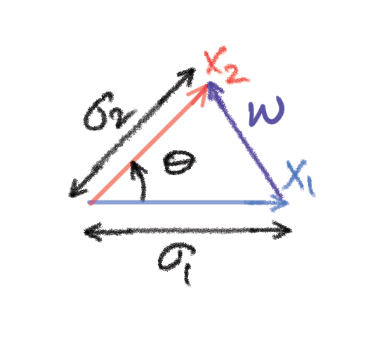
From the relationship between the vectors in the diagram, we can see that the random variable . Its variance can be calculated algebraically as . It is easily checked that this matches exactly the well-known elementary geometric relationship between the sides of a triangle: .

This vector representation is very useful for an intuitive understanding of dependencies between Gaussian random variables. In particular, the geometric concept of orthogonal projection allows us to visualize an important idea in Bayesian inference: the conditional distribution of one set of Gaussian random variables given another. This is the topic for Part 4.