In theory, we can build wireless comms over a wide range of frequencies ranging from near-DC (i.e. low frequency, very long waves e.g. 1000 mi) to ultra-violet (very high freq, very short e.g. 10-7 m). In practice, there is a small band of spectrum which is, basically, prime EM real-estate. It is easy to understand what these frequencies are and why they are so desirable based on ideas we have already been discussing.
To start from the basics: any current carrying wire generates wireless radiation i.e. functions as a transmitting antenna.
(Conversely, any piece of wire exposed to ambient EM waves can function as a receiving antenna. There is a famous reciprocity principle that asserts roughly that the properties of a receiving antenna are closely related to the transmitting properties of the same antenna. Physical/geometric structures that makes good transmitting antennas also make good receiving antennas and vice versa. We will focus on transmitters in our discussion. See Wikipedia article here for some details: reciprocity implies that antennas work equally well as transmitters or receivers, and specifically that an antenna’s radiation and receiving patterns are identical.)
Any time-varying current creates a H-field (i.e. magnetic field) around it, which generates a E-field, which generates an H-field and so forth. This is what is called an EM wave. As an aside, the idea of imagining EM fields as the result of superposition of contributions from a primary source current which produces H-fields which act like a secondary source itself producing more E- and H-fields and so forth, is a very powerful and elegant tool dating back to the 17’th century physicist Huygens and more recently popularized by celebrity scientist Richard Feynman. From Wikipedia:
In 1678, Huygens proposed that every point reached by a luminous disturbance becomes a source of a spherical wave; the sum of these secondary waves determines the form of the wave at any subsequent time.
Usually, we don’t want our metal wires in circuits acting like transmitting antennas; this represents undesirable power dissipation and produces EMI – basically EM pollution – that may mess up other nearby circuits. This is why we twist our twisted-pair wires, and shield our coax cables. The exception, of course, is wireless transmitter circuits where we want to produce a lot of radiation.
Electrically Small Antennas. Recall our definition of the corner frequency of a piece of wire as the frequency at which the electrical length of the wire is unity. At much lower frequencies, the waves are very long and the wire is said to be electrically small. And electrically short antennas are famously inefficient! From R. C. Hansen, “Fundamental limitations in antennas,” in Proc. IEEE, 1981:
With the miniaturization of components endemic in almost all parts of electronics today, it is important to recognize the limits upon size reduction of antenna elements.These are related to the basic fact that the element’s purpose is to couple to a free space wave, and the free space wavelength has not yet been miniaturized!
It is important to emphasize that this is a fundamental physical limit, rather than a shortcoming of our design methods. A very simplified intuitive explanation is as follows. Recall our earlier discussion of EM waves as E- and H-fields progressively generating each other. To get a energetic EM wave going, we need a strong source H-field generating a strong E-field. Indeed, in a propagating EM wave in free space, energy of the wave is split exactly in half between the E- and H-fields.
At low frequencies. we can have strong E-fields, or strong H-fields, but it is very hard to get both. As an example, we can make a large E-field by depositing a charge on a capacitor. However, at low frequencies, the associated charging current – and therefore the H-field – is very small. The resulting radiation is ultimately limited by the weaker of the E- and H-fields.
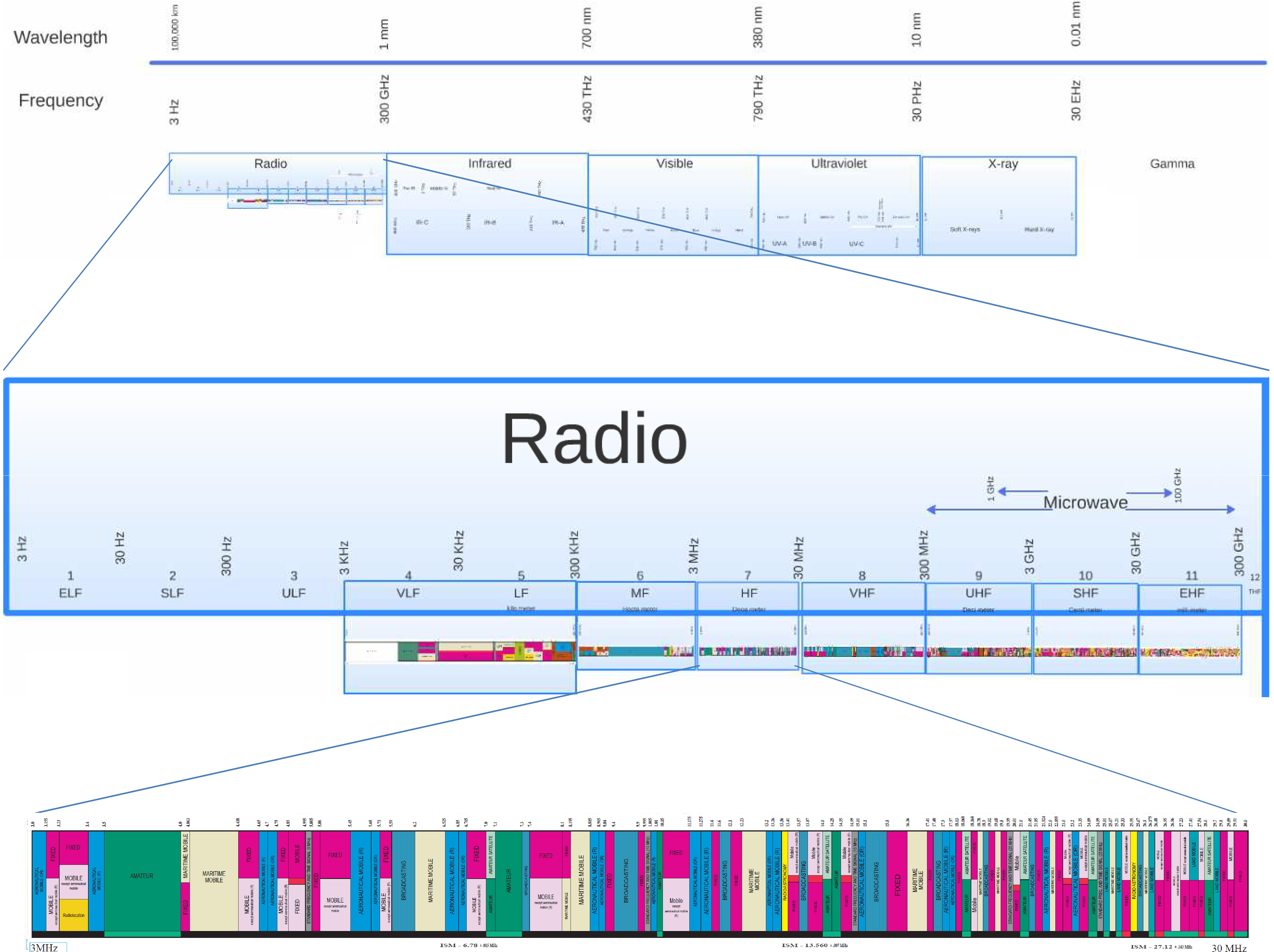
The beachfront real-estate of the EM spectrum
What frequency is high enough to efficiently generate EM waves? Recall from our discussion of transmission lines in Part 1, that propagating EM waves naturally arise when wavelengths are comparable to the physical dimensions of a circuit. The animation below shows resonance in a dipole one-half wavelength long:
 (Source: Wikipedia)
Wavelengths that are close to human-scale (λ~1 ft) are naturally the most convenient frequencies for wireless comms. The corresponding frequencies – roughly 300 MHz to 3 GHz or so – represents the most desirable real-estate in the EM spectrum. At frequencies significantly lower than this, we are in the challenging “electrically small” regime discussed above.
Subprime Real-Estate
But what about higher frequencies? By our reasoning above, it should be possible to build devices with very small form factors that can still radiate efficiently at very short wavelengths. Also, there is naturally more bandwidth available at high frequencies.
Unfortunately, these potential advantages are negated by a couple of serious drawbacks. First, circuit design is inherently challenging ay very short wavelengths. In addition to transmission line effects, various kinds of parasitic resistances and reactances that are negligible at lower frequencies become significant. Transistor gain also degrades with frequency. However, these are technological limitations, and can be expected to improve over time.
A second class of limitations is more fundamental: short waves tend to be absorbed and obstructed by objects in the physical environment that are invisible to longer waves. A simple mental model helps visualize this important phenomenon quite nicely.
What is the size of a EM wave?
“How many angels can dance on the head of a pin?” (image: Laura Guerin
Source: CK-12 Foundation):

With all appropriate disclaimers, picture EM waves as a stream of photons which are spheres with a radius equal to their wavelength. Thus a 100 MHz wave consists of long waves with photons 3 m in radius. Such long waves penetrate right through walls and other physical objects that are “thin” compared to their size. In contrast, a 10 GHz wave with photons 3 cm in size will be mostly absorbed or reflected by a concrete wall. Shorter waves in the mm-wave band are affected by even smaller objects such as dust or rain drops whose sizes are comparable to that of the photons.
In practice, waves shorter than 3 cm or so (> ~10 GHz) are limited to Line-of-Sight propagation. This makes these frequency bands inconvenient for indoor or mobile wireless comms.
It turns out that extremely short EM waves (e.g. in the visible light spectrum) do not propagate well for wireless comms, but can be caged and guided over very long distances with very high efficiency. Thus optical fiber is the medium of choice for present-day non-wireless comms applications.
Compared to radio waves, optical fiber is a nearly perfect comms medium and therefore somewhat uninteresting from a comms design perspective. Nevertheless, the physics of wave-guides presents an interesting contrast with both transmission lines and free space wireless. An intuitive discussion of wave-guides and optical fiber is a topic for Part 3.
and this does not depend at all on how other teams fare against each other!
.
or
. This number has fewer nines in it than one may expect..

 from Massey, James L. “Coding and modulation in digital communication.” Zurich Seminar on Digital Communications, 1974. Vol. 2. No. 1. 1974. There is a version of this diagram in every text including ours.
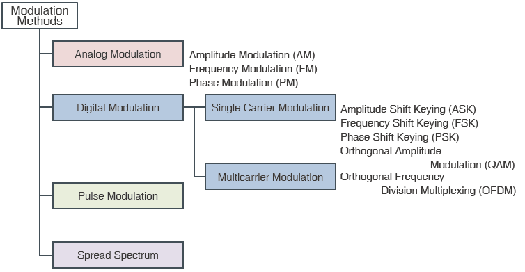
 (the I- and Q-components) relative to a carrier signal:
  .
. of the carrier signal is somewhat arbitrary, but it makes sense to choose the frequency near the center of the passband to minimize the bandwidth of the resulting baseband signals.
 has the I- and Q-components:
  .
. and the AM connection is more obvious
  .
. from
from 
 varies with the inout
  in a simple and potentially useful way. Let’s see if we can figure out what that input-output relationship is.
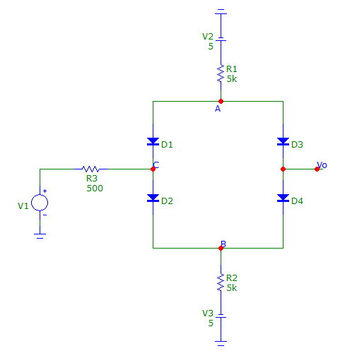
 in forward conducting mode and zero current otherwise.
 possible states for the diodes in this circuit for a given input voltage
  . Likewise, we must have
  . Note however, that there are no constraints on how low
  , and how high
  , can get.
 above node B i.e.
  .
. .
. and
and  are both off, then
  . Similarly,
  and
and  are both off, then
  .
. , we would expect
  ?
? , purely by symmetry, we would expect
  . What does this mean for the state of each of the diodes and the other node voltages?

 are both very small (ideally zero), and the gain A very large (ideally
  ). Thus, a very small voltage difference
  at the op-amp inputs can produce a large output voltage
  .
. to be whatever they need to be, to force the currents and voltage difference at the input terminals to be zero i.e.
  . In other words, the op-amp adjusts its output voltage and current in such a way that the input terminals look simultaneously like an open circuit and a short circuit! It is very elegant and almost seems magical when you set it up correctly.
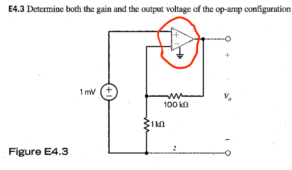
 . The op-amp then forces the output voltage
  .
.